Introduction

This post aims to review the three main forms of learning that are fundamental to the machine learning domain. If you understand terms like regression vs classification, are aware of the uses of dimensionality reduction, and know the difference between model based RL and model free RL you are not the target audience. However, feel free to read it if you want some new insight or want to refresh your knowledge.

The structure of this post is as follows. Section 1 goes over some common conventions that will be used throughout this article. Section 2 will provide an overview of the categories of tasks that ML algorithms are adept at modelling. Here, 2.1 will discuss the two forms of supervised learning, 2.2 will speak to the types of unsupervised learning, and section 2.3 will give a quick overview on the difference between model based and model free RL.

Table of Contents

• 1 - Conventions

• 2 - Types of Learning

  • 2.1 - Supervised Learning

    • 2.1.1 - Classification
    • 2.1.2 - Regression

  • 2.2 - Unsupervised Learning

    • 2.2.1 - Clustering
    • 2.2.2 - Dimensionality Reduction

  • 2.3 - Reinforcement Learning

    • 2.3.1 - Model Based RL vs Model Free RL

• 3 - Conclusion

1 - Conventions

Before we start, here are some conventions that will be used throughout the course of the article. Regardless of the category of ML you're using, you will have some data that you wish to work with, some form of information that you wish to glean from the data, and an algorithm that you want to use on it. The collection of data you are working with is referred to as the dataset, and we'll call this $X$. The dataset consists of $N$ instances of data, $x$ where each instance is a vector of length $n$ that encodes various information relevant to the problem. This is the input to the ML algorithm and is often also called a feature vector. As such $x \in \R^n$ and by extension $X \in \R^{N \times n}$. The information you are trying to glean is the output of your algorithm and this is represented as $\hat y$. The size of the vector $\hat y$ will be referred to as $m$ and it is independent of the size of $x$, it is instead based on what you are trying to learn from the data, thus $\hat y \in \R^m$. Lastly, the algorithm that is used to model the data and capture the relationship between the inputs and outputs is denoted as $f$. This forms the following formalization of what an ML model really does:

Yup! At the heart of it, an ML algorithm just learns to map an input $x$ to its corresponding output $\hat y$.

If you haven't seen the symbol $\R$ before, it represents the set of real numbers. This refers to all possible values a number can take on from $-\infty$ to $\infty$, including those that have decimal values. $X \in \R^{N \times n}$ is simply saying that $X$ is a matrix of $N$ by $n$ real numbers. Similarly, $x \in \R^n$ says that the vector $x$ consists of $n$ real numbers.

2 - Types of Learning

There mainly exist three categories of tasks for which machine learning algorithms can be leveraged. These are supervised learning, unsupervised learning, and reinforcement learning.

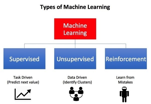
Supervised learning is useful for problems where you have a dataset that consists of pairs of input data, and the output you want from it. This could be something like historical stock data, where you predict the price an hour into the future given the current price. Training a model like this is done by pairing price data at a specific point in time with the actual price that occurred an hour after. Unsupervised learning deals more with discovering existent patterns in data. An example would be recommender systems, which cluster similar users of a service together and then provide recommendations to those users based on the preferences of others in their cluster. Finally, there is reinforcement learning a type of task where an agent is trained in an environment to maximize a given objective. This could be as simple as training an AI to play a game and achieve a high score.

2.1 - Supervised Learning

Supervised learning is applicable to tasks where we have a set of inputs and a predetermined set of outputs (known as labels) that we want with respect to the inputs. Simply put, this means that given a certain collection of data, there exists a set of feature/input vectors $x$, a set of label vectors $y$, and a relationship $g$ between the two such that $y = g(x)$. Note that here I use $y$ instead of $\hat y$. The distinction between $y$ and $\hat y$ is that $y$ refers to the true values corresponding to some input $x$ while $\hat y$ refers to the values predicted by the ML algorithm. The goal of supervised learning is to train a machine learning algorithm $f$ that models $g$ as accurately as possible by minimizing the difference between $y$ and $\hat y$. This form of learning can be used to model a wide variety of tasks including language translation, object detection, and human pose estimation.

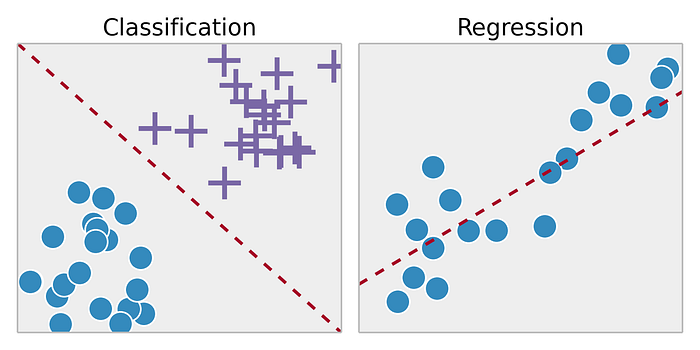
Supervised learning tasks can be split into two broad types, classification and regression. Classification tasks are those where you wish to assign an instance of data to a categorical value. This means that given an input vector, you wish to elicit a group or category that is representative of that input. An example of this could be image recognition where you classify an object that is at the center of an image. The gist of it is you're mapping a set of vectors (the pixels of an image) to a single discrete instance (the class of the object in the image).

Regression on the other hand works in the continuous domain. Here you are trying to infer some characteristic(s) with respect to the input data. An example for this sort of task is trying to predict future stock price data given past performance (trust me, this is a lot easier said than done).

2.1.1 - Classification

As mentioned above, classification tasks are those where you wish to categorize instances of data into discrete predefined sets. Since this is a form of supervised learning, you must have a dataset of inputs $x$ with an accompanying set of labels $y$; each classification problem will have a total number of classes that exist within a dataset. Here, the maximum number of classes is denoted as $l$. In most instantiations of the classification task each $x$ is only associated with a single ground truth label $y$. This means that both $\hat y, y \in \R^1$ and as such the class with the highest confidence is the class the model attributes to the input $x$. While multi-label classification (where each instance from the dataset can be associated with more than one label) does exist, that is outside the scope of this post. Here we discuss the general case of classification where $x$ belongs to a single class from a collection of 1 or more possible classes (i.e. $l \geq 1$).

Modelling this task can be accomplished using many algorithms such as logistic regression, decision trees, random forests, and neural networks. What classification algorithms learn to model is a categorical distribution that quantifies the likelihood of the input belonging to each of the possible classes. Given a well enough trained model, the class with the highest likelihood is the class the instance of data belongs to. The formalization of this kind of learning is as follows:

Here $x \in \R^n$ represents a vector of size $n$, a single instance from the dataset and $\hat y$ denotes the class the model predicts is associated with $x$. Extending this, $\hat Y \in \R^l$ is a vector where each element represents one of $l$ possible classes. Finally $p(\hat Y|x)$, which is the class probabilities $\hat Y$ given $x$, is also a vector of size $l$ and it is the output of the learning algorithm $f$. It represents a probability mass function conditioned on $x$ which quantifies the model's confidence that $x$ belongs to each of the possible classes. The properties of a probability mass function are that all elements must exist within the range 0 to 1 (inclusive), and all elements summed must equal 1.

2.1.2 - Regression

Regression is a subset of the supervised learning task that works in the continuous domain. Given an input vector $x$ and an associated set of continuous labels $y \in \R^m$ we train a model which predicts $\hat y \in \R^m$ that is as close to $y$ as possible. The key difference between regression and classification is that classification aims to assign the input data to a specific category, while regression aims to predict numeric values.

Let us once again consider the example of stock value prediction. If we're using historical OHLCV (Open High Low Close Volume) data, and we are trying to predict the price dynamics of the subsequent hour. There are two different approaches we can try; given $x \in \R^4$ as our input, we can predict a numeric value that represent the same four price factors of the next hour ($y \in \R^4$), or we can predict whether the average price of the next hour is greater than or less than the price of the current hour ($y \in \R^1$ and $l=2$). The first case is an example of regression, while the latter case is an example of classification. Again, I will highlight that is much easier said than done in the case of stock prediction. Please do not risk your own, or anyone else's money unless you know what you are doing.

2.2 - Unsupervised Learning

Now our focus shifts to unsupervised learning. Unsupervised learning algorithms do not use ground truth labels $y$ associated with the input data $x$ with which to learn a relationship $g$. In some cases, we may not even know if a relationship between the two exists at all. Instead, unsupervised algorithms aim to find existent patterns underlying the input data itself.

There are primarily two forms of unsupervised learning; the first is clustering, the second is dimensionality reduction. Clustering is to unsupervised learning, what classification is to supervised learning. Clustering is used to group similar datapoints from the dataset together, it identifies trends that are indicative of homogeneous clusters and assigns datapoints to each of them. Dimensionality reduction on the other hand is to unsupervised learning what regression is to supervised learning. It is used for projecting an input vector into a lower dimensional space. The output of a dimensionality reduction algorithm is a smaller vector that can be used to reconstruct the input again, as accurately as possible. Uses for dimensionality reduction include anomaly detection, information compression, and noise reduction.

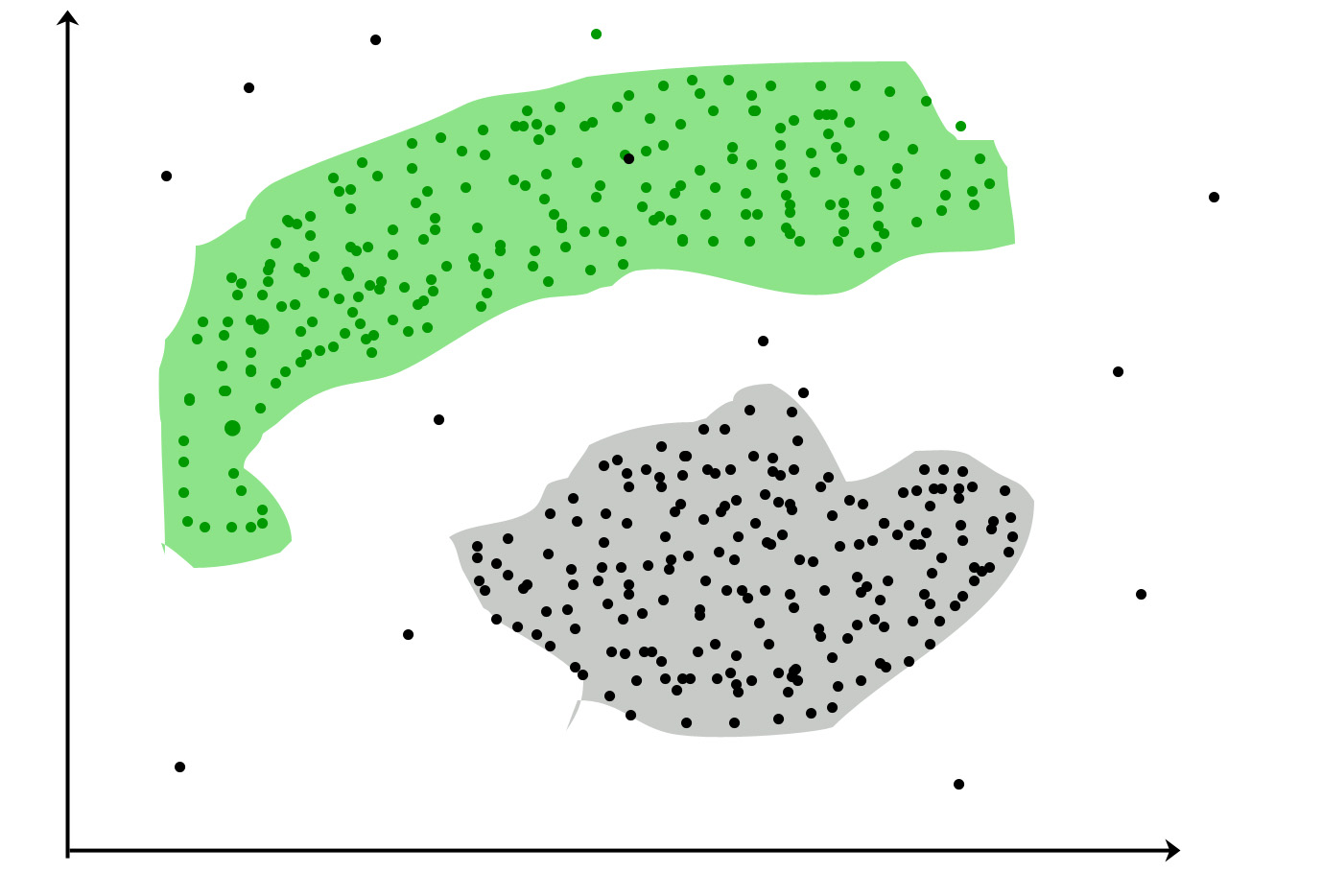
2.2.1 - Clustering

Clustering is ideal for problems where you want to group your datapoints $x$ into $m$ different clusters. It is important to note that the number of groups a clustering algorithm provides is predetermined and set before the clustering process begins; it is decided by the programmer or analyst that is using the algorithm and is constrained to $2 \leq m \ll N$ where again, $N$ refers to the total number of datapoints in your dataset $X$.

One of the biggest uses of a clustering algorithm is recommender systems. This is what websites such as Amazon, Netflix, and YouTube do when they provide shopping or video suggestions. They cluster users who have similar shopping or media consumption habits, and then recommend items to you that you haven't bought or seen based on the history of other users in your cluster.

2.2.2 - Dimensionality Reduction

Dimensionality reduction algorithms attempts to project a dataset from a high-dimensional space into a lower-dimensional space while preserving the properties of the original input. Given a dataset $X \in \R^{N \times n}$ consisting of $N$ instances $x \in \R^n$ we train an algorithm that can capture the properties of $x$ and output a latent representation $z \in \R^m$ where $m$ is defined by $0 < m < n$.

Here the metric of effectiveness would be how well $z$ can be projected back to a $n$ dimensional space. This reprojection $\hat x \in \R^n$ is then compared to $x$ itself, and the closer each $\hat x$ is to the corresponding inputs across your dataset, the better your dimensionality reduction algorithm is at capturing the relationships between the elements in the vector $x$. This can be formalized as follows:

Where $f$ is responsible for projecting $x$ into the lower dimensional space, and $f^{-1}$ is responsible for projecting it back. An example of such an algorithm is Principal Component Analysis (PCA).

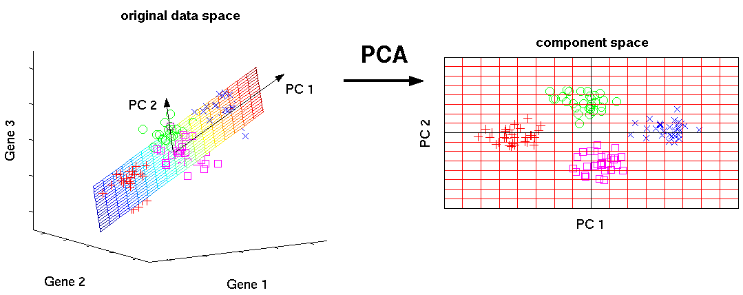
PCA is a linear dimensionality reduction algorithm performed by first calculating a covariance or correlation matrix of the dataset $X$, followed by finding the matrix's corresponding eigenvectors and eigenvalues. Here, the number of eigenvectors that are used represents the cardinality of the lower dimensional space $m$. The corresponding eigenvalues represents the values at each of the elements of $z$.

2.3 - Reinforcement Learning

The final form of learning is reinforcement learning. Reinforcement learning is ideal for problems that can be defined as a Markov Decision Process (MDP). An MDP consists of two main elements; the first is the agent, which is an autonomous decision making entity that aims to achieve a given goal. The second element is the environment, which is everything outside of the agent. This consists of the world that the agent exists within, as well as other agents in the same environment.

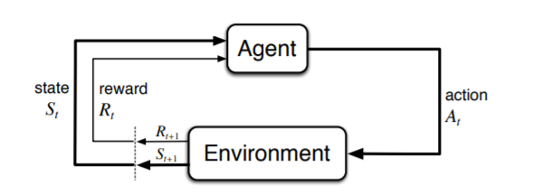
An MDP codifies the interactions between an agent and its environment. The agent receives the current state of the environment $S_t$ as input and decides on an action $A_t$ to take. Following this action, the state of the environment will change; the agent then gets this new state $S_{t+1}$, and a reward $R_{t+1}$ that represents how succesful the agent has been at fulfilling its objective thus far. This interaction then continues on until some end state is reached.

The previous kinds of learning we have discussed primarily use the domain of the outputs as the main distinction within those forms of learning; with classification and clustering working in the discrete/categorical domain, while regression and dimensionality reduction work in the continuous domain. Reinforcement learning has no such distinction, here the outputs of the ML algorithm used by the agent to make decisions (referred to as its policy $\Pi$) can be discrete, continuous, or both. The primary distinction is whether there exists a model of the environment the algorithm is working in.

2.3.1 - Model Based RL vs Model Free RL

When we speak of model based vs. model free reinforcement learning, we are not talking about if the agent is using an ML model for its policy. Instead, we are talking about whether the agent has a model to predict the environment's next state before it takes an action. It leverages the environment model by simulating various scenarios using this model to predict the possible actions it can take, as well as the change in the environment's state, and based on this information it decides what to do. This model could be a direct mathematical model that captures the dynamics of the environment, or it could be an entirely separate ML model that has been trained to capture the environment.

An example of a situation where you would use model based RL is when you're training an agent to play a board game like chess or Go. Deepmind's AlphaGo system uses a game model to decide on the optimal strategy each time it makes a decision; it simulates many possible moves, and the likely moves by the opponent in response before finalizing an action. Model free RL is used in cases where creating an environment model is not tractable. If a model is available, it is almost always better to use model based RL methods.

3 - Conclusion

This post discussed the 3 main categories of machine learning, these categories include supervised learning, unsupervised learning, and reinforcement learning. It then summarized the distinctions within these forms of learning and which form of learning is ideal for which situation.

While I spoke of the three types of ML in terms of their differences, it is worth noting that most ML pipelines actually combine the various kinds to make a full fledged machine learning system. For example a model based RL algorithm could potentially use a supervised learning algorithm as its environment model; similarly, a dimensionality reduction algorithm can be used to compress the feature space of the original inputs which is then subsequently fed to a supervised learning algorithm to make a prediction. This could be considered a form of feature engineering, which is modifying the original set of features to make it easier to discover underlying patterns.

This completes my post on types of ML algorithms. I hope you learned something new, and feel free to comment or email me with questions. Stay tuned for more in this series to introduce newcomers to the world of machine learning!